Notes from Frank’s Microrealms online workshop

To enable LED control, make pins PB_6 and PB_7, add these lines to the runGame function in “realm.c”:

RCC->IOPENR = (1 << 2) + (1 << 1) + (1 << 0); // set bits 0,1,2 to enable ports A,B,C
pinMode(GPIOB, 7, 1); // Make PB_7 an output
pinMode(GPIOB, 6, 1); // Make PB_6 an output

Add this to the code that runs when you find an elixir of health – i.e. a ‘h’ on the map:

GPIOB->ODR |= (1u << 6); // LED on (set pin PB_6 to 3.3V)
delay(100000);
GPIOB->ODR &= ~(1u << 6); // LED off (set pin PB_6 to 0V)

Add this to the code that runs when you find a potion of strength – i.e. an ‘s’ on the map:

GPIOB->ODR |= (1u << 7); // LED on (set pin PB_7 to 3.3V)
delay(100000);
GPIOB->ODR &= ~(1u << 7); // LED off (set pin PB_7 to 0V)

To enable audio, we need to generate a square wave signal from an output pin (we’ll use pin PA_0). Copy the following lines from from our previous SysTick example into the runGame function in “realm.c”.

pinMode(GPIOA,0,1); // Make PORTA Bit 0 an output
SysTick->LOAD = 15999;   // 16MHz / 16000 = 1kHz
SysTick->CTRL = 7;       // enable systick counting and interrupts, use core clock
enable_interrupts();

Then copy the following lines, also from the SysTick example into “realm.c”:

void SysTick_Handler(void)
{
    static int ms_counter = 0;
    GPIOA->ODR ^= 1; // Toggle Port A bit 0
    ms_counter ++; // another millisecond has passed
    if (ms_counter == 1000) // 1 second passed ?
    {
        ms_counter = 0; // zero millisecond counter
        GPIOA->ODR ^= 2; // toggle LED
    }
}

Add this to “realm.c”:

volatile uint32_t CycleCount = 0; // global variable to count down note duration

void playNote(int Frequency, int Duration)
{
	uint32_t LoadValue;
	LoadValue = 16000000 / (2 * Frequency);
	SysTick->LOAD = LoadValue;
	CycleCount = (Frequency * Duration) / 1000;
	while(CycleCount > 0); // wait for note to finish
}

Update the SysTick_Handler function in “realm.c” as follows:

void SysTick_Handler(void)
{
	if (CycleCount > 0)
	{
		GPIOA->ODR ^= 1; // Toggle Port A bit 0
		CycleCount--;
	}
	else
	{
		GPIOA->ODR &= ~1; // turn off speaker
	}
}

As an example, insert the following lines after the showRealm function call in “realm.c” (around line 64) to play a little audio jingle:

PlayNote(200, 100);
PlayNote(400, 100);
PlayNote(800, 100);
PlayNote(1600, 100);

You could try creating functions like…

void startupJingle()
void battleStartJingle()

Or try adding some ASCII art for different game events, etc.

Posted in Uncategorized | Leave a comment

RoadRunner Assignment

Objective

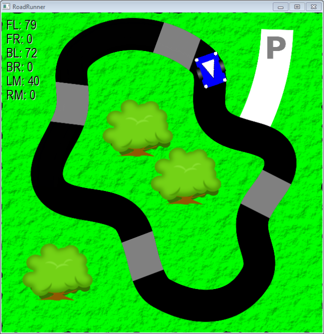
The objective of this assignment is to write a MATLAB program (i.e. an M-file) called “drive.m” which controls the RoadRunner simulator robot in real time, guiding it along the track.

RoadRunner

Deadline and Assessment

The deadline for this assignment is 5pm on Friday 11th December 2015.

The assessment will comprise two parts:

  1. The code you submit – how well it works, how clear it is, how neatly it is presented.
  2. Your understanding – based on your participation in this week’s class, how you solve the problem, questions I ask you about your solution, questions I ask you about MATLAB programming in general.

The grade you can expect will depend on how far you get with the problem. As a rough guide:

  1. To get a basic pass, you just need to get the robot driving around the track reliably and make sure the code you submit is neatly presented with self-explanatory variable names, correct indentation and plenty of clear comments. Obviously, you need to understand it too – and I’ll be checking!
  2. To get a better grade, I would like to see the robot driving around the track, but stopping for a couple of seconds on each of the grey patches on the road before driving on. Even better would be to print out a message each time a grey patch is encountered saying how many have been encountered up to that point.
  3. If you want to do really well, do all of the above and then, after counting 6 grey patches, turn into the white driveway and park on top of the letter P.

Submitting your program

You will submit only one M-file to me – “drive.m” – which contains your final solution.

Download the RoadRunner simulator

You’re very welcome to install the RoadRunner simulator onto your own PC. You can download the RoadRunner simulator here:

To test your program, you will also need MATLAB or Octave. If you’re working on your own PC, I recommend downloading Octave. It’s free software, easy to install and should run your M-file without modification. You can download it here:

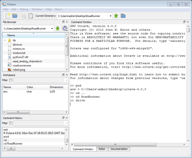
There is an executable installer for Octave on Windows, but I don’t use it myself. I just recommend downloading the zip file, octave-4.0.0_0.zip, and extracting the folder it contains to a convenient location such as your desktop (that’s where I keep the octave-4.0.0 folder). To start Octave, just go into the octave-4.0.0 folder and double click “octave.bat”.

Octave_drive

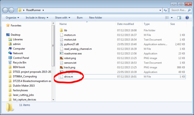
RoadRunner_folder

Posted in Uncategorized | Leave a comment

Box Counter Challenge

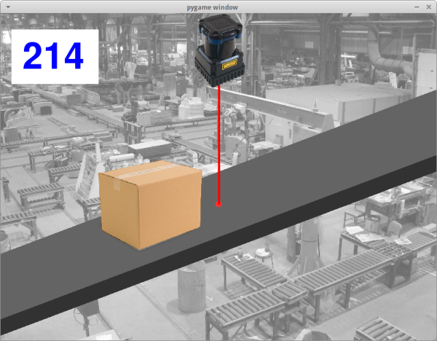
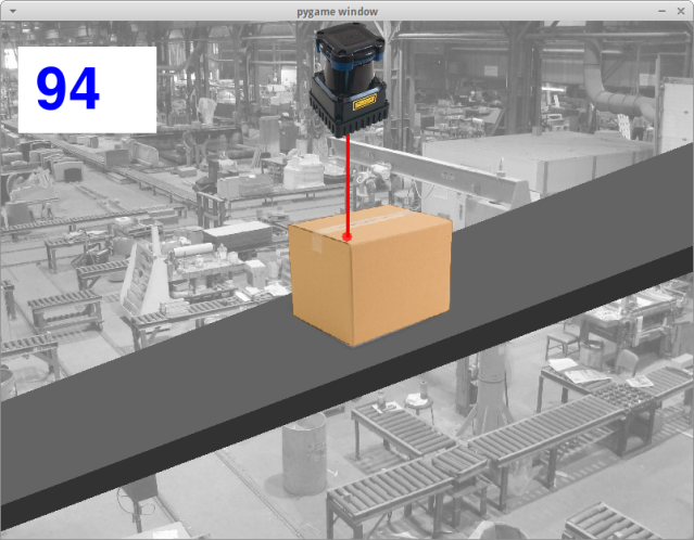
In this challenge, you need to write a MATLAB program to count boxes

Screenshot_2015-11-12_09-53-20

Screenshot_2015-11-12_09-53-36

Posted in Uncategorized | Leave a comment

Final Assignment – “Face Painter”

The objective in this assignment is to write a MATLAB program (“face.m”) which creates a PGM file containing the following image of a face:

face

The basic characteristics of the image are:

  • Image width: 320 px
  • Image height: 240 px
  • Background colour: light grey (pixel value 200)
  • Face stroke colour: black (pixel value 0)
  • Face fill colour: white (pixel value 255)
  • Outer radius of face: 100 px
  • Stroke width: 20 px

By “stroke”, I just mean a line or curve that forms part of the face.

The deadline for this assignment is the end of this week’s class (Thursday 23rd April 2015). You will be able to work on it during the class, but remember that we will also be doing the functions quiz, which will take up about 30 minutes of the 2-hour class. You should therefore be arriving to class with at least a rough solution to the Face Painter problem. I can try to help you iron out any remaining issues at that point, but please bear in mind that I will be assessing your understanding during the class, so it’s in your own interest to show me that you can work independently and that you’re not relying on me too much.

Submission

You will submit your final M-file “face.m” to me by email not later than Thursday 23rd April 2015, together with any additional M-files that it relies on, such as “drawrectangle.m” or whatever else you may have used in your solution.

A related example: Stripes

To solve this problem, you will probably use some of the approaches we discussed in class before the Easter break. To remind you what we were doing before Easter and to get you started on the face problem, here’s a related (but simpler) example, which draws the following image of three stripes:

stripes

To create that image, I wrote an M-file called “stripes.m” which contains the code shown below:

%
% stripes.m - Draws a 320x240 px image with light
% grey background and three vertical black stripes
%   
% Written by Ted Burke - last modified 18-4-2015
%

% Create a blank light grey image (all pixels = 200)
img = 200 * ones(240,320);

% Draw three vertical black stripes
img = drawrectangle(img, 0, 50, 50, 20, 140);
img = drawrectangle(img, 0, 150, 50, 20, 140);
img = drawrectangle(img, 0, 250, 50, 20, 140);

% Write the image to a PGM file
pgmwrite(img);

You will notice that the program uses a function called “drawrectangle” which I also wrote. This function adds a rectangle to an image. The position, size and colour of the rectangle are all passed as arguments (input values) to the function. The function returns the modified image (which is stored in a MATLAB matrix with 240 rows and 320 columns). The drawrectangle function is saved in a second M-file, called “drawrectangle.m”, which contains the code shown below:

%
% drawrectangle.m - Draws a rectangle of the specified colour at the
% specified coordinates in the array "image".
%
% Arguments are:
%
%   image  : the array (matrix) that stores the image
%   grey   : the shade of grey of the rectangle
%   left   : the x coordinate of the left side of the rectangle
%   top    : the y coordinate of the top of the rectangle
%   width  : the width of the rectangle in pixels
%   height : the height of the rectangle in pixels
%   
% Written by Ted Burke - last modified 18-4-2015
%

function image = drawrectangle(image, grey, left, top, width, height)
    % outer loop iterated over the rows in the image
    y = top;
    while y < top + height
        % inner loop iterates over the pixels in the current row
        x = left;
        while x < left + width
            % this sets the colour of the pixel at the current x,y point
            image(y,x) = grey;
            x = x + 1;
        end
        y = y + 1;
    end
end

Finally, the program also uses the same “pgmwrite” function that we used in class before Easter. In case you don’t still have that M-file, here’s the complete code, which should be saved as “pgmwrite.m”:

%
% pgmwrite.m - MATLAB function to write a matrix
% of pixel values to a greyscale PGM image file.
%
% Written by Ted Burke - last updated 12-3-2015
%
 
function pgmwrite(pixels)
    % Check matrix dimensions which will determine
    % the width and height of the image
    s = size(pixels);
    height = s(1);
    width = s(2);
     
    % Open a file for writing
    fid = fopen('image.pgm','w');
     
    % Write the PGM image header to the file
    fprintf(fid,'P2\n');
    fprintf(fid,'%d %d\n', width, height);
    fprintf(fid,'255\n');
     
    % Write the pixel values from the matrix into
    % the file
    y = 1;
    while y <= height
        x = 1;
        while x <= width
            fprintf(fid, '%03d ', pixels(y,x));
            x = x + 1;
        end
        fprintf(fid, '\n');
        y = y + 1;
    end
     
    % Close the file
    fclose(fid);
end

To run the “stripes” example, you should place the three files “stripes.m”, “drawrectangle.m” and “pgmwrite.m” into the same folder. Then, in MATLAB, navigate to the same folder and type “stripes” to run the program.

Hints for the Face Painter problem

There are lots of ways you could solve the face drawing problem, but the approach I took was to create another new function called “drawcircle” which was saved in an M-file called “drawcircle.m”. If you decide to take this approach, you’ll need to write the function yourself, but to give you a bit of a hint, this was the comment from the start of my “drawcircle.m”:

%
% drawcircle.m - Draws a circle of the specified colour at the
% specified coordinates in the array "image".
%
% Arguments are:
%
%	image  : the array (matrix) that stores the image
%	grey   : the shade of grey of the rectangle
%	cx     : the x coordinate of the circle centre
%	cy     : the y coordinate of the circle centre
%	r      : the circle radius
%	
% Written by Ted Burke - last modified 18-4-2015
%

I then wrote the file “face.m” which created a blank grey image and added a number of circles and rectangles using the “drawcircle” and “drawrectangle” functions.

If your require clarification on any aspect of the assignment, you can either leave a comment on this post or email me and I’ll do my best to address your query. By all means contact me if you’re stuck on some aspect of the problem too, but keep in mind that I’ll be hoping to see evidence that you’re getting making a serious effort to get stuck into the problem yourself.

Posted in Uncategorized | Leave a comment

pgmwrite.m

%
% pgmwrite.m - MATLAB function to write a matrix
% of pixel values to a greyscale PGM image file.
%
% Written by Ted Burke - last updated 12-3-2015
%

function pgmwrite(pixels)
    % Check matrix dimensions which will determine
    % the width and height of the image
    s = size(pixels);
    height = s(1);
    width = s(2);
    
    % Open a file for writing
    fid = fopen('image.pgm','w');
    
    % Write the PGM image header to the file
    fprintf(fid,'P2\n');
    fprintf(fid,'%d %d\n', width, height);
    fprintf(fid,'255\n');
    
    % Write the pixel values from the matrix into
    % the file
    y = 1;
    while y <= height
        x = 1;
        while x <= width
            fprintf(fid, '%03d ', pixels(y,x));
            x = x + 1;
        end
        fprintf(fid, '\n');
        y = y + 1;
    end
    
    % Close the file
    fclose(fid)
end
Posted in Uncategorized | Leave a comment

pgmwrite.m – a MATLAB function to write a matrix to a PGM file

Note: To run IrfanView (which displays PGM image files) on the School network, browse to the following file and double click it:

Y:\OldApps\tburke\IrfanView\i_view32.exe
%
% pgmwrite.m - MATLAB function to write a matrix
% of pixel values to a greyscale PGM image file.
%
% Written by Ted Burke - last updated 12-3-2015
%

function pgmwrite(pixels)
    % Check matrix dimensions which will determine
    % the width and height of the image
    s = size(pixels);
    height = s(1);
    width = s(2);
    
    % Open a file for writing
    fid = fopen('image.pgm','w');
    
    % Write the PGM image header to the file
    fprintf(fid,'P2\n');
    fprintf(fid,'%d %d\n', width, height);
    fprintf(fid,'255\n');
    
    % Write the pixel values from the matrix into
    % the file
    y = 1;
    while y <= height
        x = 1;
        while x <= width
            fprintf(fid, '%03d ', pixels(y,x));
            x = x + 1;
        end
        fprintf(fid, '\n');
        y = y + 1;
    end
    
    % Close the file
    fclose(fid)
end

Here’s an example of a short MATLAB script which creates a matrix containing pixel values and then uses the above function to write the pixels into a PGM file:

%
% drawpicture.m - Create a PGM image file using pgmwrite.m
%

% Create a matrix of the desired image dimensions
% In this case, height is 200 and width is 300...
p = zeros(200,300);

% Calculate the pixel values using a nested while loop
y = 1;
while y <= 200
    x = 1;
    while x <= 300
        if y == x
            p(y,x) = 255;
        else
            p(y,x) = 100;
        end
        x = x + 1;
    end
    y = y + 1;
end

% Write pixels to a PGM image file
pgmwrite(p);

When the resulting image file “image.pgm” is opened in IrfanView, it appears as follows:

irfanview_screenshot

Posted in Uncategorized | Leave a comment

DT066 Computing assignment: “Trolley Tracker”

General Information

  • The deadline for this assignment is 10pm on Wednesday 4rd March 2015.
  • You will submit a single file called “trolleytracker.m” which contains your program. You will submit the file to me by email.
  • Please note that the primary method of assessment in this assignment is the interview which I will carry out with each of you after submission (probably on Thursday 5th March 2015). The purpose of the interview is to assess your level of knowledge and understanding of MATLAB programming in general, and especially the program you have submitted. Experience has shown that students who are struggling with programming assignments sometimes feel tempted to submit code they do not actually understand. However, since you will be interviewed on your own submitted code, it would be highly inadvisable to do that in this assignment.
  • The interview will focus primarily on the program you submitted, but you may also be asked some general programming questions on topics such as: variables, MATLAB matrices, if statements, while loops, printing text and numbers, file input and output, etc.

The Trolley Tracker problem

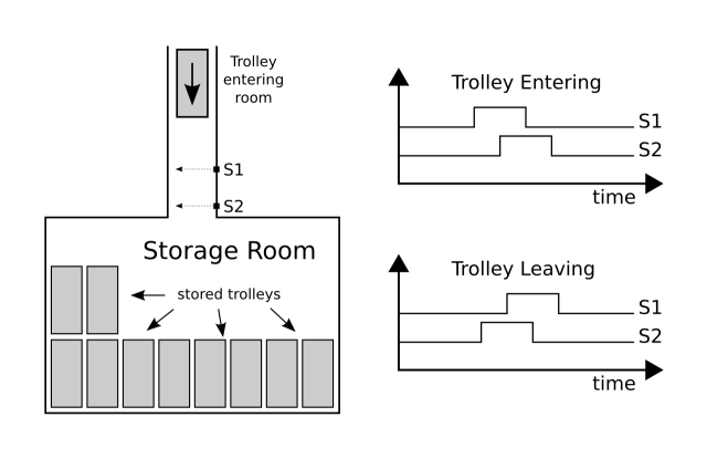
The objective of this assignment is to write a MATLAB program to track the number of trolleys stored in a storage room in a factory by analysing data recorded from two ultrasonic distance sensors mounted on the wall of the corridor leading to the storage room. The storage room can accommodate up to 16 trolleys. At the beginning of each working day, the room is empty.

  • Both sensors are mounted at the same height on the same wall. The sensors are 1 metre apart.
  • Each sensor faces directly across the corridor.
  • The longer the distance to the nearest object, the lower the sensor output.
  • The shorter the distance to the nearest object, the higher the sensor output.
  • Each trolley is exactly 2 m in length and passes the sensors at a constant velocity between 1.0 and 1.5 m/s.
  • Each sensor therefore outputs a positive pulse as a trolley passes.
  • Trolleys entering the room trigger Sensor 1 first and sensor 2 second.
  • Trolleys leaving the room trigger Sensor 2 first and sensor 1 second.
  • Each passing trolley generates two pulses – one from each sensor – which overlap in time.
  • When a trolley enters the room, the Sensor 1 pulse leads the Sensor 2 pulse.
  • When a trolley leaves the room, the Sensor 2 pulse leads the Sensor 1 pulse.

trolley_storage_room

The sensors are sampled at 10 Hz (i.e. each sensor measures the distance 10 times per second) and the data are recorded to a CSV file over the course of the 8-hour working day. Your program must do the following:

  1. Load the data from one of these CSV files into a MATLAB matrix and analyse the readings to count the number of trolleys entering and leaving the room.
  2. Assuming there are no trolleys in the room at the start of each day, print the number of trolleys present in the room at the end of the working day.
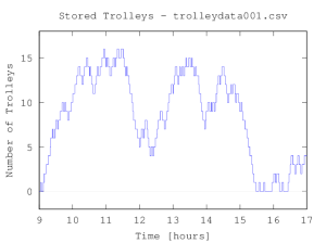
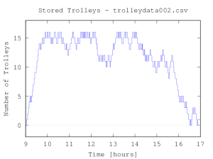
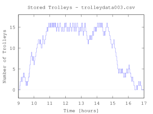
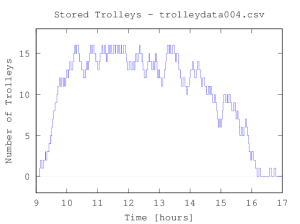
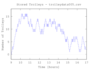
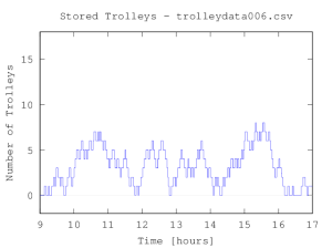
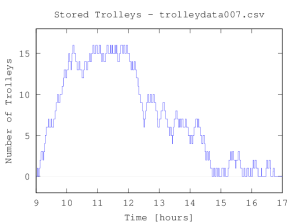
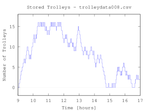
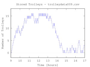
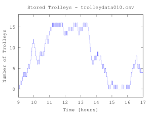
  3. Plot a graph of the number of trolleys stored in the room over the course of the day. Examples plots are shown below. Your program should be clear and professionally presented.
  4. Your program should add an appropriate title and axis labels to each graph.

Example data

I have created ten example CVS data files, which can be downloaded as a single zip archive from the following link:

The following list provides the final trolley count for each of the ten example data files:

Filename Final Count
trolleydata001.csv 4
trolleydata002.csv 1
trolleydata003.csv 0
trolleydata004.csv 0
trolleydata005.csv 2
trolleydata006.csv 1
trolleydata007.csv 0
trolleydata008.csv 2
trolleydata009.csv 3
trolleydata010.csv 4

A trolley count plot for each of the ten example data files is shown below:

trolleydata001

trolleydata002

trolleydata003

trolleydata004

trolleydata005

trolleydata006

trolleydata007

trolleydata008

trolleydata009

trolleydata010

Posted in Uncategorized | Leave a comment

Incomplete example code for ECG Challenge (DT066 Computing)

This was the example ECG challenge code we discussed at the end of today’s class. Note that this is NOT a complete solution! It certainly won’t count the correct number of heart beats as it is shown below.

%
% heartbeats.m - Estimate heartrate from an ECG recording
% Written by Ted Burke - last updated 29-1-2015
%

% Load ECG data from CSV file, starting at row 3
data = csvread('samples.csv', 3);

% Extract the second column of data and store it in ecg
ecg = data(:,2);

% Display a graph of the ECG signal
plot(ecg)

% Create a counter variable to count our way through the data
n = 1;

% Create a variable to count the heartbeats
beats = 0;

while n < 7679
    if ecg(n) > 0.6
        beats = beats + 1;
    end
    
    n = n + 1
end

% Display number of heartbeats
disp(beats)

The sample ECG data can be downloaded by clicking here.

Posted in Uncategorized | Leave a comment

Worked examples from today’s lecture

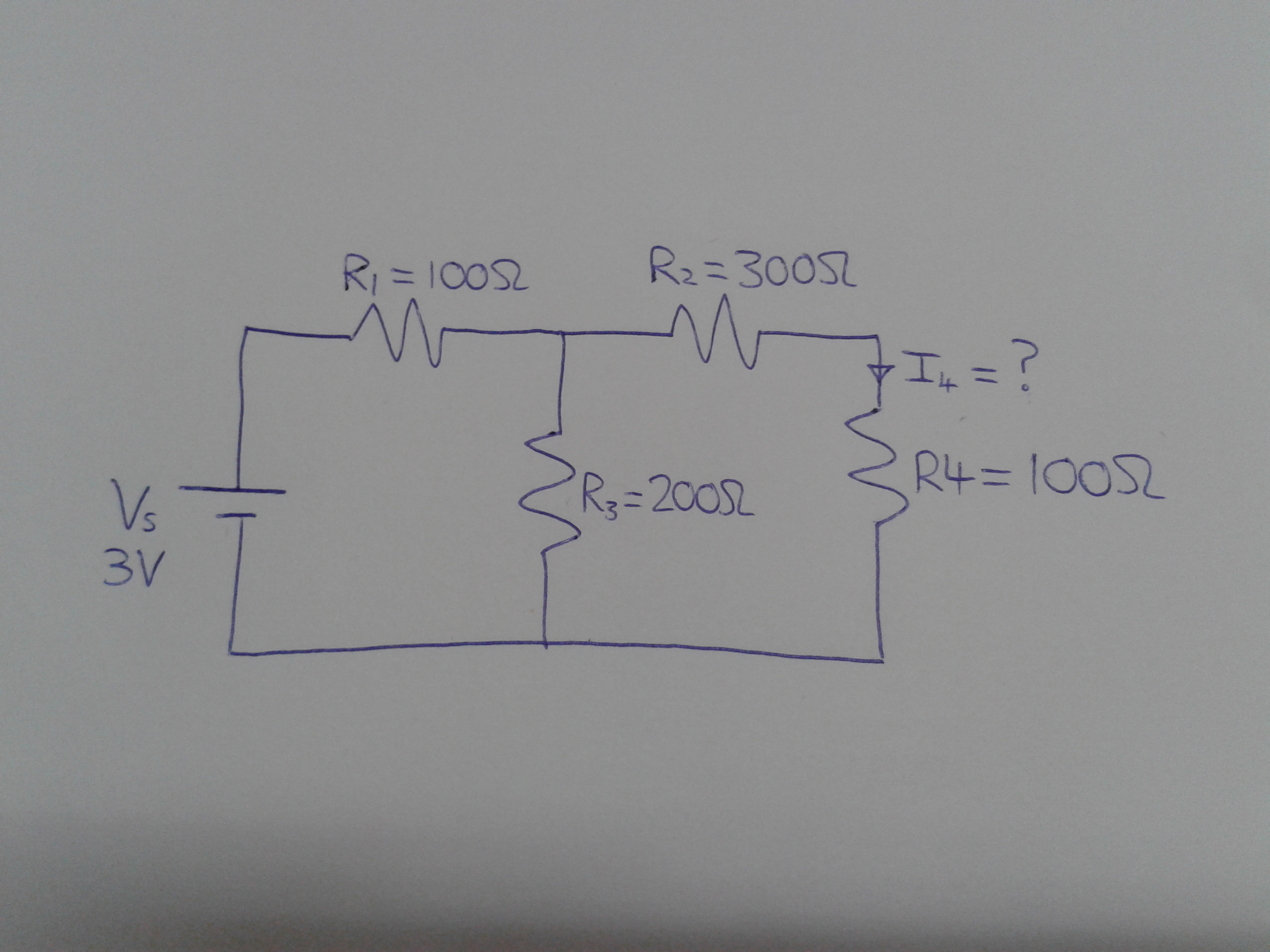
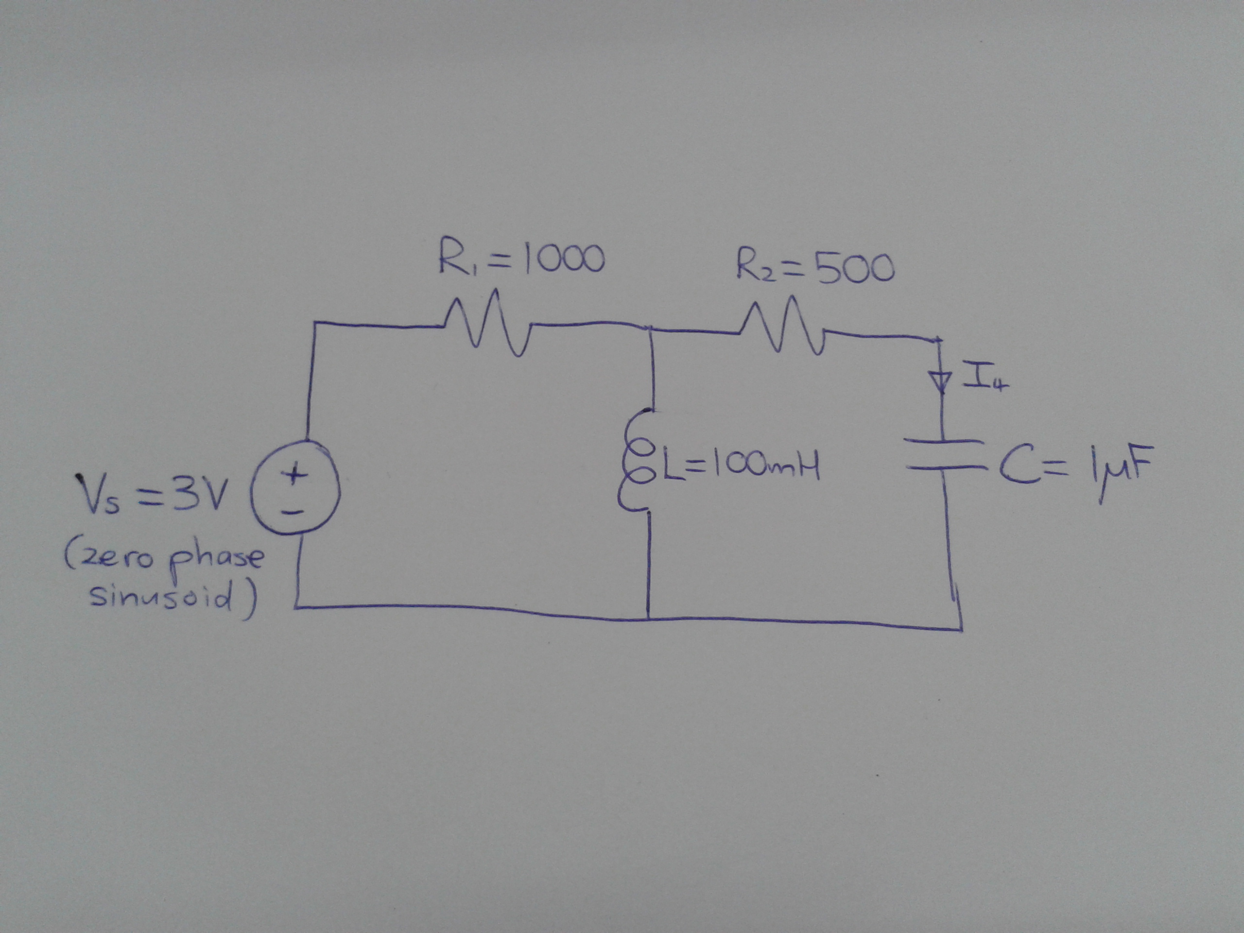
DC circuit example:

2014-03-11 15.56.45

%
% DC circuit worked example
%

% supply voltage
Vs = 3;

% original resistors
R1 = 100;
R2 = 300;
R3 = 200;
R4 = 100;

% Equivalent resistor for R2 & R4 in series
R5 = R2 + R4;

% Equivalent resistor for R3 || R5 (parallel)
R6 = (R3 * R5) / (R3 + R5);

% Find voltage across R3
V3 = Vs * (R6 / (R1 + R6));

% Finally, calculate the current I4
I4 = V3 / R5

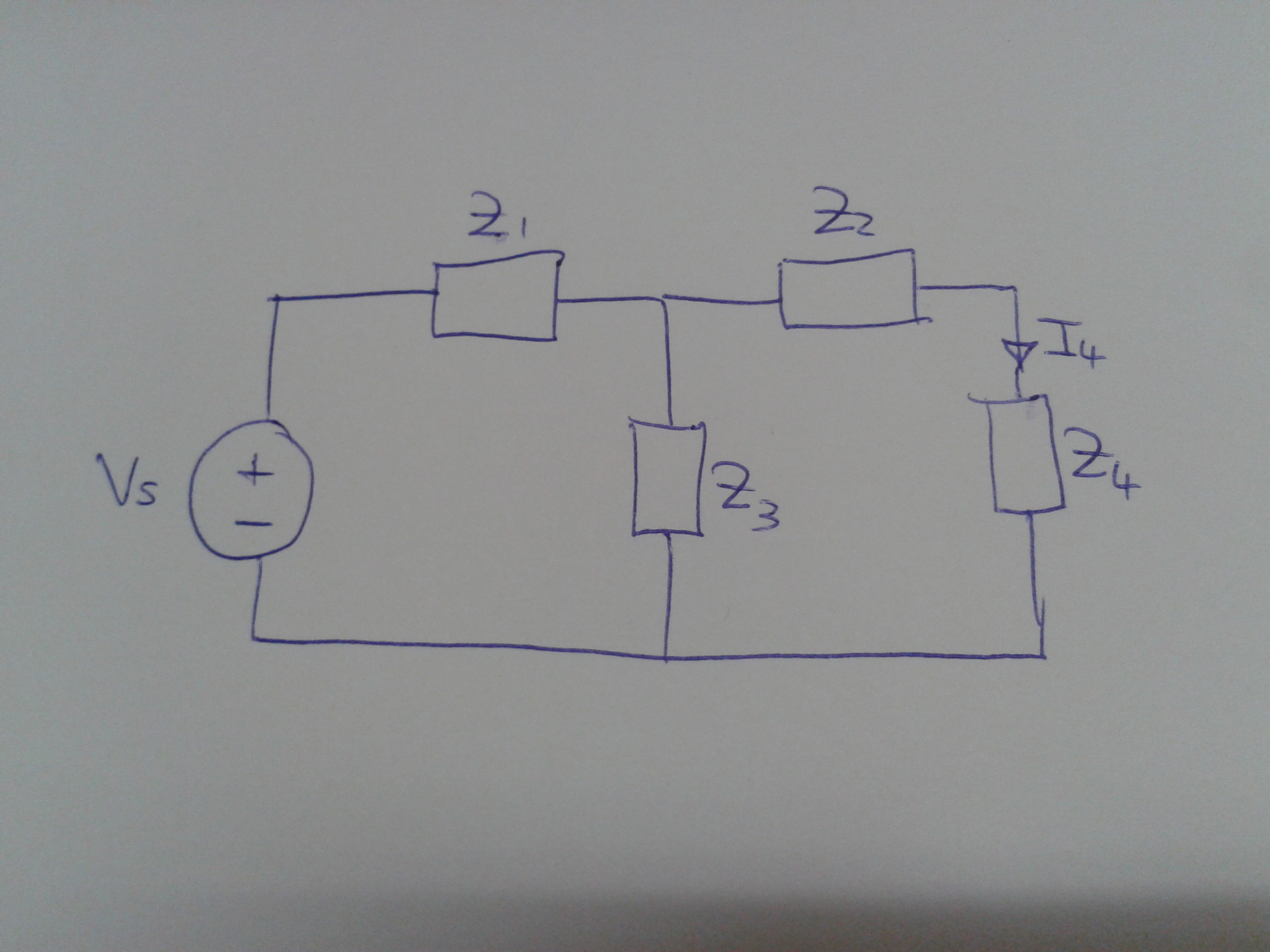
AC circuit example:

2014-03-11 15.59.47

2014-03-11 16.00.46

%
% AC circuit worked example
%

% create variable for j (square root of -1)
j = 0 + 1j;

% supply voltage
Vs = 3 + 0*j;
f = 1000;
w = 2 * pi * f;

% inductor and capacitor
L = 100e-3;
C = 1e-6;

% original impedances
Z1 = 1000;
Z2 = 500;
Z3 = j * w * L;
Z4 = 1 / (j * w * C);

% Equivalent impedance for Z2 & Z4 in series
Z5 = Z2 + Z4;

% Equivalent impedance for Z3 || Z5 (parallel)
Z6 = (Z3 * Z5) / (Z3 + Z5);

% Find voltage (as a phasor) across Z3
V3 = Vs * (Z6 / (Z1 + Z6));

% Finally, calculate the current I4 (as a phasor)
I4 = V3 / Z5

disp(abs(I4))
disp(angle(I4))

To plot phasor diagram, you can use the MATLAB function below. Copy the following code into a new M-file and save it in the same folder as the above M-files.

%
% phasors.m - written by Ted Burke 25-2-2014
% This function plots an array of complex numbers as phasors
%

function phasors(Z,labels)
	figure
	hold on
	
	% Calculate a suitable axis limit based on phasors
	m = 1.5 * max([real(Z) imag(Z)]);
	
	% Create a new figure window
	figure
	hold on
	
	% Plot phasors
	h = quiver(0*real(Z),0*imag(Z),real(Z),imag(Z),'filled');
	set(h, 'autoscalefactor', 1.0, 'linewidth', 3.0)
	
	% Phasor labels
	for n = 1:(size(labels))(1)
		text(real(1.1*Z(n)),imag(1.1*Z(n)),labels(n,:));
	end
	
	% Draw horizontal and vertical axis lines
	plot([-m m],[0 0])
	plot([0 0],[-m m])
	
	% Set axis limits and aspect ratio
	axis([-m,m,-m,m], 'square')
end

To plot a phasor diagram of complex variables Vs and Vc (for example):

phasors([Vs Vc], ['Vs';'Vc'])
Posted in Uncategorized | Leave a comment

Phasor diagram example for MATLAB / Octave

First create the following utility function (save as “phasors.m”) for plotting phasor diagrams:

%
% phasors.m - written by Ted Burke 25-2-2014
% This function plots an array of complex numbers as phasors
%

function phasors(Z)
	figure
	hold on
	
	% Calculate a suitable axis limit based on phasors
	m = 1.2 * max([abs(real(Z)) abs(imag(Z))]);
	
	% Create a new figure window
	figure
	hold on
	
	% Plot phasors one at a time
	quiver(0*real(Z),0*imag(Z),real(Z),imag(Z));
	
	% Draw horizontal and vertical axis lines
	plot([-m m],[0 0])
	plot([0 0],[-m m])
	
	% Set axis limits and aspect ratio
	axis([-m,m,-m,m], 'square')
end

Now, a simple example calculation for a series RC circuit with a 10V AC power supply:

% RCphasors.m - An RC circuit example

% create a variable j equal to sqrt(-1)
j = 0 + 1j;

% frequency in Hz and angular frequency in rad/s
f = 50;
w = 2*pi*f;

% supply voltage has magnitude 10V and zero phase angle
% i.e. at its maximum value at t=0
Vs = 10;

% Component values
R = 1e3;
C = 1e-6;

% impedance of capacitor
Zc = 1 / (j*w*C);

% total equivalent impedance of series R and C
Zeq = R + Zc;

% Calculate current
I = Vs / Zeq;

% Calculate capacitor and resistor voltages
Vc = I * Zc;
Vr = I * R;

% Display current magnitude and phase
disp 'Current magnitude (A):'
disp (abs(I))
disp 'Current phase angle (rad):'
disp (angle(I))

% Plot a phasor diagram (scale I to make it visible)
phasors([Vs 1000*I])

RCphasors

RCphasors_console

Posted in Uncategorized | 2 Comments